Fit a Second Order Polynomial to the given data. Curve fitting Polynomial Regression

Got data that doesn’t make a straight line? No worries! Polynomial regression helps find the right curve for your numbers.

Let’s learn how to use it for fitting a second-order curve to your data – perfect for spotting trends in a snap.

Polynomial Regression Example

Let’s say you have the following data points:

x	1.0	2.0	3.0	4.0
y	6.0	11.0	18.0	27.0

Solution:

Let Y = a₁ + a₂x + a₃x²    ( 2^nd order polynomial ).

Here, m = 3  ( because to fit a curve we need at least 3 points ).

Since the order of the polynomial is 2, therefore we will have 3 simultaneous equations as below.

1. Polynomial Regression Formula

To learn more, see what is Polynomial Regression

2. Evaluate Formula

Now we have to evaluate the values that are required according to the above equations.

Let us find the value of x2, x3, x4, yx, and yx2.

x	y	x2	x3	x4	yx	yx2
1.0	6.0	1	1	1	6	6
2.0	11.0	4	9	16	22	44
3.0	18.0	9	16	81	54	162
4.0	27.0	16	36	256	108	432
∑xi=10	∑yi=62	∑x2=364	∑x3=524	∑x4=354	∑yx=190	∑yx2=644

3. Substitute Values

Put the values in the above 3 equations as below.

4a₁ + 10a₂ + 30a₃ = 62   …. ( 1 )

10a₁ + 30a₂ + 100a₃ = 190  …. ( 2 )

30a₁ + 100a₂ + 354a₃ = 644  … ( 3 )

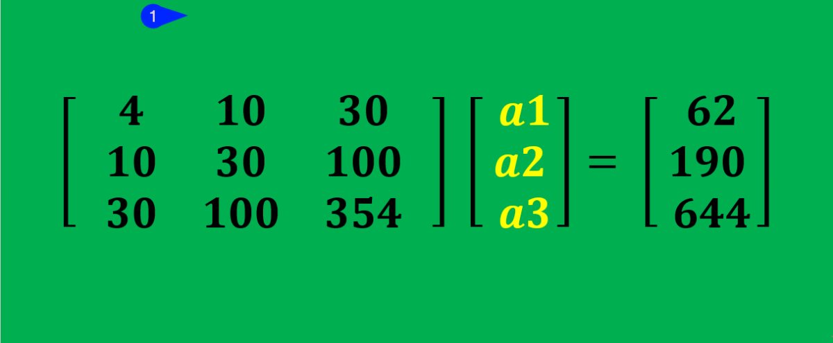
4. Make Matrix

In order to solve the above 3 simultaneous equations, we will write the above equations in the form of matrices as below.

5. Use Matrix Elimination

By using matrix elimination techniques, you can solve for the coefficients a, b, and c.

Now by using back substitution, we can find the values of a1, a2, and a3.

Here, 4a3 = 4 , a3 = 1
And, a2 + 5a3 = 7 , a2 = 2
Also, a1 + 2.5a2 + 7.5a3 = 15.5 , a1 = 3
Therefore, a1 = 3, a2 = 2, a3 = 1.

6. Final Equation

The Quadratic equation becomes: Y = 3 + 2x + x2, or

Sol:- Y = x² + 2x + 3

This is your second-order polynomial regression equation that closely matches your given data points!

Suggestion:

1. Newtons Interpolation
2. Lagrange’s Interpolation
3. Bisection method
4. Regula falsi method
5. Linear Regression

Conclusion

In simple words, polynomial regression helps us find the right curve that fits our data points, even when they don’t play nicely with a straight line.

It’s a bit of math magic that lets us make predictions and understand trends in our data.

Just remember, not every problem needs a fancy high-degree polynomial – sometimes, a simple line works best.